Data Structures and Algorithms (DSA) is a fundamental part of Computer Science that teaches you how to think and solve complex problems systematically.
Using the right data structure and algorithm makes your program run faster, especially when working with lots of data.
The word 'algorithm' comes from 'al-Khwarizmi', named after a Persian scholar who lived around year 800.
The concept of algorithmic problem-solving can be traced back to ancient times, long before the invention of computers.
The study of Data Structures and Algorithms really took off with the invention of computers in the 1940s, to efficiently manage and process data.
Today, DSA is a key part of Computer Science education and professional programming, helping us to create faster and more powerful software.
What are Data Structures?
A data structure is a way to store data.
We structure data in different ways depending on what data we have, and what we want to do with it.
First, let's consider an example without computers in mind, just to get the idea.
If we want to store data about people we are related to, we use a family tree as the data structure. We choose a family tree as the data structure because we have information about people we are related to and how they are related, and we want an overview so that we can easily find a specific family member, several generations back.
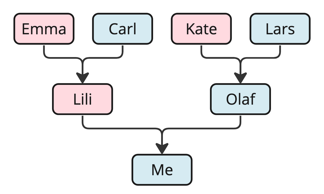
With such a family tree data structure visually in front of you, it is easy to see, for example, who my mother's mother is - it is 'Emma,' right? But without the links from child to parents that this data structure provides, it would be difficult to determine how the individuals are related.
Data structures give us the possibility to manage large amounts of data efficiently for uses such as large databases and internet indexing services.
Data structures are essential ingredients in creating fast and powerful algorithms. They help in managing and organizing data, reduce complexity, and increase efficiency.
In Computer Science there are two different kinds of data structures.
- Primitive Data Structures are basic data structures provided by programming languages to represent single values, such as integers, floating-point numbers, characters, and booleans.
- Abstract Data Structures are higher-level data structures that are built using primitive data types and provide more complex and specialized operations. Some common examples of abstract data structures include arrays, linked lists, stacks, queues, trees, and graphs.
What are Algorithms?
An algorithm is a set of step-by-step instructions to solve a given problem or achieve a specific goal.
A cooking recipe written on a piece of paper is an example of an algorithm, where the goal is to make a certain dinner. The steps needed to make a specific dinner are described exactly.
When we talk about algorithms in Computer Science, the step-by-step instructions are written in a programming language, and instead of food ingredients, an algorithm uses data structures.
Algorithms are fundamental to computer programming as they provide step-by-step instructions for executing tasks. An efficient algorithm can help us to find the solution we are looking for, and to transform a slow program into a faster one.
By studying algorithms, developers can write better programs.
Algorithm examples:
- Finding the fastest route in a GPS navigation system;
- Navigating an airplane or a car (Cruise Control);
- Finding what users search for (Search Engine);
- Sorting, for example sorting movies by rating;
Theory and Terminology
- Algorithm. A set of step-by-step instructions to solve a specific problem.
- Data Structure. A way of organizing data so it can be used efficiently. Common data structures include arrays, linked lists, and binary trees.
- Time Complexity. A measure of the amount of time an algorithm takes to run, depending on the amount of data the algorithm is working on.
- Space Complexity. A measure of the amount of memory an algorithm uses, depending on the amount of data the algorithm is working on.
- Big O Notation. A mathematical notation that describes the limiting behavior of a function when the argument tends towards a particular value or infinity.
- Recursion. A programming technique where a function calls itself.
- Divide and Conquer. A method of solving complex problems by breaking them into smaller, more manageable sub-problems, solving the sub-problems, and combining the solutions. Recursion is often used when using this method in an algorithm.
- Brute Force. A simple and straight forward way an algorithm can work by simply trying all possible solutions and then choosing the best one.
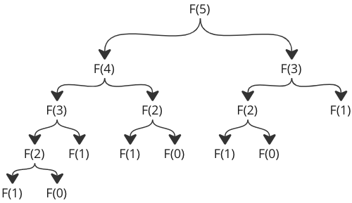
Fibonacci Numbers
The Fibonacci numbers are very useful for introducing algorithms, so before we continue, here is a short introduction to Fibonacci numbers.
The Fibonacci numbers are named after a 13th century Italian mathematician known as Fibonacci.
The two first Fibonacci numbers are 0 and 1, and the next Fibonacci number is always the sum of the two previous numbers, so we get 0, 1, 1, 2, 3, 5, 8, 13, 21, ...
- The Fibonacci Number Algorithm
To generate a Fibonacci number, all we need to do is to add the two previous Fibonacci numbers.
The Fibonacci numbers is a good way of demonstrating what an algorithm is. We know the principle of how to find the next number, so we can write an algorithm to create as many Fibonacci numbers as possible.
Below is the algorithm to create the 20 first Fibonacci numbers.
1. Start with the two first Fibonacci numbers 0 and 1.
a. Add the two previous numbers together to create a new Fibonacci number.
b. Update the value of the two previous numbers.
2. Do point a and b above 18 times.
- Loops vs. Recursion
To show the difference between loops and recursion, we will implement solutions to find Fibonacci numbers in three different ways:
- An implementation of the Fibonacci algorithm above using a for loop.
- An implementation of the Fibonacci algorithm above using recursion.
- Finding the nth Fibonacci number using recursion.
- Implementation Using a For Loop
It can be a good idea to list what the code must contain or do before programming it:
- Two variables to hold the previous two Fibonacci numbers
- A for loop that runs 18 times
- Create new Fibonacci numbers by adding the two previous ones
- Print the new Fibonacci number
- Update the variables that hold the previous two fibonacci numbers
Using the list above, it is easier to write the program:
prev2 = 0
prev1 = 1

print(prev2)
print(prev1)

for fibo in range(18):
    newFibo = prev1 + prev2
    print(newFibo)
    prev2 = prev1
    prev1 = newFibo
- Implementation Using Recursion
Recursion is when a function calls itself.
To implement the Fibonacci algorithm we need most of the same things as in the code example above, but we need to replace the for loop with recursion.
To replace the for loop with recursion, we need to encapsulate much of the code in a function, and we need the function to call itself to create a new Fibonacci number as long as the produced number of Fibonacci numbers is below, or equal to, 19.
Our code looks like this:
print(0)
print(1)
count = 2

def fibonacci(prev1, prev2):
    global count

    if count <= 19:
        newFibo = prev1 + prev2
        print(newFibo)
        prev2 = prev1
        prev1 = newFibo
        count += 1
        fibonacci(prev1, prev2)
    else:
        return

fibonacci(1, 0)
- Finding The nth Fibonacci Number Using Recursion
To find the nth Fibonacci number we can write code based on the mathematic formula for Fibonacci number n:
F(n) = F(n - 1) + F(n - 2)
This just means that for example the 10th Fibonacci number is the sum of the 9th and 8th Fibonacci numbers.
Note: This formula uses a 0-based index. This means that to generate the 20th Fibonacci number, we must write F(19).
When using this concept with recursion, we can let the function call itself as long as n is less than, or equal to, 1. If n ≤ 1 it means that the code execution has reached one of the first two Fibonacci numbers 1 or 0.
The code looks like this:
def F(n):
    if n <= 1:
        return n
    else:
        return F(n - 1) + F(n - 2)

print(F(19))
Notice that this recursive method calls itself two times, not just one. This makes a huge difference in how the program will actually run on our computer. The number of calculations will explode when we increase the number of the Fibonacci number we want. To be more precise, the number of function calls will double every time we increase the Fibonacci number we want by one.
Just take a look at the number of function calls for F(5):
To better understand the code, here is how the recursive function calls return values so that F(5) returns the correct value in the end:
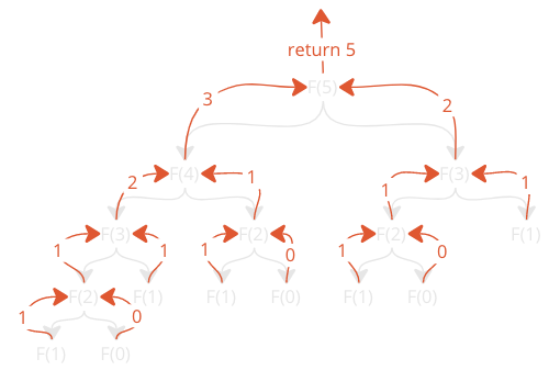
There are two important things to notice here: The amount of function calls, and the amount of times the function is called with the same arguments.
So even though the code is fascinating and shows how recursion work, the actual code execution is too slow and ineffective to use for creating large Fibonacci numbers.
Arrays
An array is a data structure used to store multiple elements.
Arrays are indexed, meaning that each element in the array has an index, a number that says where in the array the element is located.
- Algorithm: Find The Lowest Value in an Array
Let's create our first algorithm using the array data structure.
Below is the algorithm to find the lowest number in an array.
- Go through the values in the array one by one.
- Check if the current value is the lowest so far, and if it is, store it.
- After looking at all the values, the stored value will be the lowest of all values in the array.
- Implementation
Before implementing the algorithm using an actual programming language, it is usually smart to first write the algorithm as a step-by-step procedure.
If you can write down the algorithm in something between human language and programming language, the algorithm will be easier to implement later because we avoid drowning in all the details of the programming language syntax.
- Create a variable 'minVal' and set it equal to the first value of the array.
- Go through every element in the array.
- If the current element has a lower value than 'minVal', update 'minVal' to this value.
- After looking at all the elements in the array, the 'minVal' variable now contains the lowest value.
You can also write the algorithm in a way that looks more like a programming language if you want to, like this:
Variable 'minVal' = array[0]
For each element in the array
    If current element < minVal
        minVal = current element
Note: The two step-by-step descriptions of the algorithm we have written above can be called 'pseudocode'. Pseudocode is a description of what a program does, using language that is something between human language and a programming language.
After we have written down the algorithm, it is much easier to implement the algorithm in a specific programming language:
my_array = [7, 12, 9, 4, 11]
minVal = my_array[0]

for i in my_array:
    if i < minVal:
        minVal = i

print('Lowest value:', minVal)
- Time Complexity
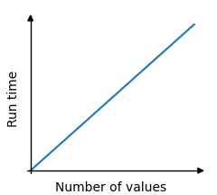
When exploring algorithms, we often look at how much time an algorithm takes to run relative to the size of the data set.
In the example above, the time the algorithm needs to run is proportional, or linear, to the size of the data set. This is because the algorithm must visit every array element one time to find the lowest value. The loop must run 5 times since there are 5 values in the array. And if the array had 1000 values, the loop would have to run 1000 times.
Bubble Sort
Bubble Sort is an algorithm that sorts an array from the lowest value to the highest value.
The word 'Bubble' comes from how this algorithm works, it makes the highest values 'bubble up'.
- How it works
- Go through the array, one value at a time.
- For each value, compare the value with the next value.
- If the value is higher than the next one, swap the values so that the highest value comes last.
- Go through the array as many times as there are values in the array.
- Implementation
To implement the Bubble Sort algorithm in a programming language, we need:
- An array with values to sort.
- An inner loop that goes through the array and swaps values if the first value is higher than the next value. This loop must loop through one less value each time it runs.
- An outer loop that controls how many times the inner loop must run. For an array with n values, this outer loop must run n-1 times.
The resulting code looks like this:
my_array = [64, 34, 25, 12, 22, 11, 90, 5]
n = len(my_array)

for i in range(n-1):
    for j in range(n-i-1):
        if my_array[j] > my_array[j+1]:
            my_array[j], my_array[j+1] = my_array[j+1], my_array[j]

print("Sorted array:", my_array)
- Improvement
The Bubble Sort algorithm can be improved a little bit more.
Imagine that the array is almost sorted already, with the lowest numbers at the start, like this for example:
my_array = [7, 3, 9, 12, 11]
In this case, the array will be sorted after the first run, but the Bubble Sort algorithm will continue to run, without swapping elements, and that is not necessary.
If the algorithm goes through the array one time without swapping any values, the array must be finished sorted, and we can stop the algorithm, like this:
my_array = [7, 3, 9, 12, 11]
n = len(my_array)

for i in range(n-1):
    swapped = False
    for j in range(n-i-1):
        if my_array[j] > my_array[j+1]:
            my_array[j], my_array[j+1] = my_array[j+1], my_array[j]
            swapped = True
    if not swapped:
        break

print("Sorted array:", my_array)
- Time Complexity
The Bubble Sort algorithm loops through every value in the array, comparing it to the value next to it. So for an array of n values, there must be n such comparisons in one loop.
And after one loop, the array is looped through again and again n times.
This means there are n*n comparisons done in total, so the time complexity for Bubble Sort is:
O(n2)
The graph describing the Bubble Sort time complexity looks like this:
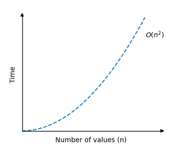
As you can see, the run time increases really fast when the size of the array is increased.
Luckily there are sorting algorithms that are faster than this, like Quicksort, that we will look at later.
Selection Sort
The Selection Sort algorithm finds the lowest value in an array and moves it to the front of the array.
The algorithm looks through the array again and again, moving the next lowest values to the front, until the array is sorted.
- How it works
- Go through the array to find the lowest value.
- Move the lowest value to the front of the unsorted part of the array.
- Go through the array again as many times as there are values in the array.
- Implementation
To implement the Selection Sort algorithm in a programming language, we need:
- An array with values to sort.
- An inner loop that goes through the array, finds the lowest value, and moves it to the front of the array. This loop must loop through one less value each time it runs.
- An outer loop that controls how many times the inner loop must run. For an array with n values, this outer loop must run n-1 times.
The resulting code looks like this:
my_array = [64, 34, 25, 5, 22, 11, 90, 12]
n = len(my_array)

for i in range(n-1):
    min_index = i
    for j in range(i+1, n):
        if my_array[j] < my_array[min_index]:
            min_index = j
    min_value = my_array.pop(min_index)
    my_array.insert(i, min_value)

print("Sorted array:", my_array)
- Shifting Problem
The Selection Sort algorithm can be improved a little bit more.
The Selection Sort algorithm can be improved a little bit more.
In the code above, the lowest value element is removed, and then inserted in front of the array.
Each time the next lowest value array element is removed, all following elements must be shifted one place down to make up for the removal.
These shifting operation takes a lot of time, and we are not even done yet! After the lowest value (5) is found and removed, it is inserted at the start of the array, causing all following values to shift one position up to make space for the new value, like the image below shows.
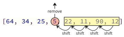
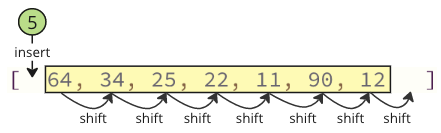
Note: You will not see these shifting operations happening in the code if you are using a high level programming language such as Python or Java, but the shifting operations are still happening in the background. Such shifting operations require extra time for the computer to do, which can be a problem.
- Solution: Swap Values
Instead of all the shifting, swap the lowest value (5) with the first value (64) like below.
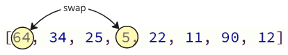
We can swap values like the image above shows because the lowest value ends up in the correct position, and it does not matter where we put the other value we are swapping with, because it is not sorted yet.
Here is an implementation of the improved Selection Sort, using swapping:
my_array = [64, 34, 25, 12, 22, 11, 90, 5]
n = len(my_array)

for i in range(n):
    min_index = i
    for j in range(i+1, n):
        if my_array[j] < my_array[min_index]:
            min_index = j
    my_array[i], my_array[min_index] = my_array[min_index], my_array[i]

print("Sorted array:", my_array)
- Time Complexity
Selection Sort sorts an array of n values.
On average, about n/2 elements are compared to find the lowest value in each loop.
And Selection Sort must run the loop to find the lowest value approximately n times.
We get time complexity:

As you can see, the run time is the same as for Bubble Sort: The run time increases really fast when the size of the array is increased.
Insertion Sort
The Insertion Sort algorithm uses one part of the array to hold the sorted values, and the other part of the array to hold values that are not sorted yet.
The algorithm takes one value at a time from the unsorted part of the array and puts it into the right place in the sorted part of the array, until the array is sorted.
- How it works
- Take the first value from the unsorted part of the array.
- Move the value into the correct place in the sorted part of the array.
- Go through the unsorted part of the array again as many times as there are values.
- Implementation
To implement the Insertion Sort algorithm in a programming language, we need:
- An array with values to sort.
- An outer loop that picks a value to be sorted. For an array with n values, this outer loop skips the first value, and must run n-1 times.
- An inner loop that goes through the sorted part of the array, to find where to insert the value. If the value to be sorted is at index i, the sorted part of the array starts at index 0 and ends at index i-1.
The resulting code looks like this:
my_array = [64, 34, 25, 12, 22, 11, 90, 5]
n = len(my_array)

for i in range(1, n):
    insert_index = i
    current_value = my_array.pop(i)
    for j in range(i-1, -1, -1):
        if my_array[j] > current_value:
            insert_index = j
    my_array.insert(insert_index, current_value)

print("Sorted array:", my_array)
- Improvement
Insertion Sort can be improved a little bit more.
The way the code above first removes a value and then inserts it somewhere else is intuitive. It is how you would do Insertion Sort physically with a hand of cards for example. If low value cards are sorted to the left, you pick up a new unsorted card, and insert it in the correct place between the other already sorted cards.
The problem with this way of programming it is that when removing a value from the array, all elements above must be shifted one index place down:
And when inserting the removed value into the array again, there are also many shift operations that must be done: all following elements must shift one position up to make place for the inserted value:
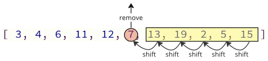
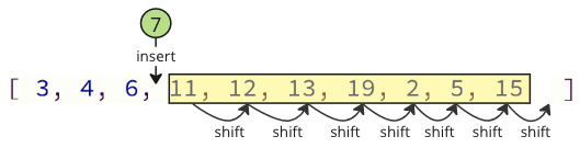
These shifting operations can take a lot of time, especially for an array with many elements.
Hidden memory shifts: You will not see these shifting operations happening in the code if you are using a high-level programming language such as Python or JavaScript, but the shifting operations are still happening in the background. Such shifting operations require extra time for the computer to do, which can be a problem.
- Improved Solution
We can avoid most of these shift operations by only shifting the values necessary:
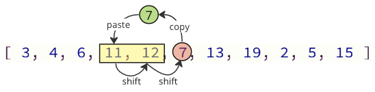
In the image above, first value 7 is copied, then values 11 and 12 are shifted one place up in the array, and at last value 7 is put where value 11 was before.
The number of shifting operations is reduced from 12 to 2 in this case.
This improvement is implemented in the example below:
my_array = [64, 34, 25, 12, 22, 11, 90, 5]
n = len(my_array)

for i in range(1, n):
    insert_index = i
    current_value = my_array[i]
    for j in range(i-1, -1, -1):
        if my_array[j] > current_value:
            my_array[j+1] = my_array[j]
            insert_index = j
        else:
            break
    my_array[insert_index] = current_value

print("Sorted array:", my_array)
What is also done in the code above is to break out of the inner loop. That is because there is no need to continue comparing values when we have already found the correct place for the current value.
- Time Complexity
Insertion Sort sorts an array of n values.
On average, each value must be compared to about n/2 other values to find the correct place to insert it.
Insertion Sort must run the loop to insert a value in its correct place approximately n times.
We get time complexity for Insertion Sort:
For Insertion Sort, there is a big difference between best, average and worst case scenarios.
Quicksort
As the name suggests, Quicksort is one of the fastest sorting algorithms.
The Quicksort algorithm takes an array of values, chooses one of the values as the 'pivot' element, and moves the other values so that lower values are on the left of the pivot element, and higher values are on the right of it.
In this tutorial the last element of the array is chosen to be the pivot element, but we could also have chosen the first element of the array, or any element in the array really.
Then, the Quicksort algorithm does the same operation recursively on the sub-arrays to the left and right side of the pivot element. This continues until the array is sorted.
Recursion is when a function calls itself.
After the Quicksort algorithm has put the pivot element in between a sub-array with lower values on the left side, and a sub-array with higher values on the right side, the algorithm calls itself twice, so that Quicksort runs again for the sub-array on the left side, and for the sub-array on the right side. The Quicksort algorithm continues to call itself until the sub-arrays are too small to be sorted.
- How it works
- Choose a value in the array to be the pivot element.
- Order the rest of the array so that lower values than the pivot element are on the left, and higher values are on the right.
- Swap the pivot element with the first element of the higher values so that the pivot element lands in between the lower and higher values.
- Do the same operations (recursively) for the sub-arrays on the left and right side of the pivot element.
- Implementation
To write a 'quickSort' method that splits the array into shorter and shorter sub-arrays we use recursion. This means that the 'quickSort' method must call itself with the new sub-arrays to the left and right of the pivot element.
To implement the Quicksort algorithm in a programming language, we need:
- An array with values to sort.
- A quickSort method that calls itself (recursion) if the sub-array has a size larger than 1.
- A partition method that receives a sub-array, moves values around, swaps the pivot element into the sub-array and returns the index where the next split in sub-arrays happens.
The resulting code looks like this:
def partition(array, low, high):
    pivot = array[high]
    i = low - 1

    for j in range(low, high):
        if array[j] <= pivot:
            i += 1
            array[i], array[j] = array[j], array[i]

    array[i+1], array[high] = array[high], array[i+1]
    return i+1

def quicksort(array, low=0, high=None):
    if high is None:
        high = len(array) - 1

    if low < high:
        pivot_index = partition(array, low, high)
        quicksort(array, low, pivot_index-1)
        quicksort(array, pivot_index+1, high)

my_array = [64, 34, 25, 12, 22, 11, 90, 5]
quicksort(my_array)

print("Sorted array:", my_array)
- Time Complexity
The worst case scenario for Quicksort is O(n2). This is when the pivot element is either the highest or lowest value in every sub-array, which leads to a lot of recursive calls. With our implementation above, this happens when the array is already sorted.
But on average, the time complexity for Quicksort is actually just O(nlogn), which is a lot better than for the previous sorting algorithms we have looked at. That is why Quicksort is so popular.
Below you can see the significant improvement in time complexity for Quicksort in an average scenario O(nlogn), compared to the previous sorting algorithms Bubble, Selection and Insertion Sort with time complexity O(n2):
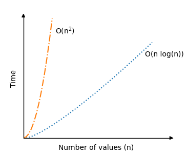
The recursion part of the Quicksort algorithm is actually a reason why the average sorting scenario is so fast, because for good picks of the pivot element, the array will be split in half somewhat evenly each time the algorithm calls itself. So the number of recursive calls do not double, even if the number of values n double.
Counting Sort
The Counting Sort algorithm sorts an array by counting the number of times each value occurs.
Counting Sort does not compare values like the previous sorting algorithms we have looked at, and only works on non negative integers.
Furthermore, Counting Sort is fast when the range of possible values k is smaller than the number of values n.
- How it works
- Create a new array for counting how many there are of the different values.
- Go through the array that needs to be sorted.
- For each value, count it by increasing the counting array at the corresponding index.
- After counting the values, go through the counting array to create the sorted array.
- For each count in the counting array, create the correct number of elements, with values that correspond to the counting array index.
- Conditions
These are the reasons why Counting Sort is said to only work for a limited range of non-negative integer values:
- Integer values: Counting Sort relies on counting occurrences of distinct values, so they must be integers. With integers, each value fits with an index (for non negative values), and there is a limited number of different values, so that the number of possible different values k is not too big compared to the number of values n.
- Non negative values: Counting Sort is usually implemented by creating an array for counting. When the algorithm goes through the values to be sorted, value x is counted by increasing the counting array value at index x. If we tried sorting negative values, we would get in trouble with sorting value -3, because index -3 would be outside the counting array.
- Limited range of values: If the number of possible different values to be sorted k is larger than the number of values to be sorted n, the counting array we need for sorting will be larger than the original array we have that needs sorting, and the algorithm becomes ineffective.
- Implementation
To implement the Counting Sort algorithm in a programming language, we need:
- An array with values to sort.
- A 'countingSort' method that receives an array of integers.
- An array inside the method to keep count of the values.
- A loop inside the method that counts and removes values, by incrementing elements in the counting array.
- A loop inside the method that recreates the array by using the counting array, so that the elements appear in the right order.
One more thing: We need to find out what the highest value in the array is, so that the counting array can be created with the correct size. For example, if the highest value is 5, the counting array must be 6 elements in total, to be able count all possible non negative integers 0, 1, 2, 3, 4 and 5.
The resulting code looks like this:
def countingSort(arr):
    max_val = max(arr)
    count = [0] * (max_val + 1)

    while len(arr) > 0:
        num = arr.pop(0)
        count[num] += 1

    for i in range(len(count)):
        while count[i] > 0:
            arr.append(i)
            count[i] -= 1

    return arr

unsortedArr = [4, 2, 2, 6, 3, 3, 1, 6, 5, 2, 3]
sortedArr = countingSort(unsortedArr)

print("Sorted array:", sortedArr)
- Time Complexity
How fast the Counting Sort algorithm runs depends on both the range of possible values k and the number of values n.
In general, time complexity for Counting Sort is O(n+k).
In a best case scenario, the range of possible different values k is very small compared to the number of values n and Counting Sort has time complexity O(n).
But in a worst case scenario, the range of possible different values k is very big compared to the number of values n and Counting Sort can have time complexity O(n2) or even worse.
The plot below shows how much the time complexity for Counting Sort can vary.
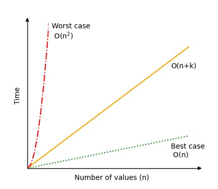
As you can see, it is important to consider the range of values compared to the number of values to be sorted before choosing Counting Sort as your algorithm. Also, as mentioned at the top of the page, keep in mind that Counting Sort only works for non negative integer values.
Radix Sort
The Radix Sort algorithm sorts an array by individual digits, starting with the least significant digit (the rightmost one).
The radix (or base) is the number of unique digits in a number system. In the decimal system we normally use, there are 10 different digits from 0 till 9.
Radix Sort uses the radix so that decimal values are put into 10 different buckets (or containers) corresponding to the digit that is in focus, then put back into the array before moving on to the next digit.
Radix Sort is a non comparative algorithm that only works with non negative integers.
- How it works
- Start with the least significant digit (rightmost digit).
- Sort the values based on the digit in focus by first putting the values in the correct bucket based on the digit in focus, and then put them back into array in the correct order.
- Move to the next digit, and sort again, like in the step above, until there are no digits left.
- Stable Sorting
Radix Sort must sort the elements in a stable way for the result to be sorted correctly.
A stable sorting algorithm is an algorithm that keeps the order of elements with the same value before and after the sorting. Let's say we have two elements "K" and "L", where "K" comes before "L", and they both have value "3". A sorting algorithm is considered stable if element "K" still comes before "L" after the array is sorted.
It makes little sense to talk about stable sorting algorithms for the previous algorithms we have looked at individually, because the result would be same if they are stable or not. But it is important for Radix Sort that the the sorting is done in a stable way because the elements are sorted by just one digit at a time.
So after sorting the elements on the least significant digit and moving to the next digit, it is important to not destroy the sorting work that has already been done on the previous digit position, and that is why we need to take care that Radix Sort does the sorting on each digit position in a stable way.
- Implementation
To implement the Radix Sort algorithm we need:
- An array with non negative integers that needs to be sorted.
- A two dimensional array with index 0 to 9 to hold values with the current radix in focus.
- A loop that takes values from the unsorted array and places them in the correct position in the two dimensional radix array.
- A loop that puts values back into the initial array from the radix array.
- An outer loop that runs as many times as there are digits in the highest value.
The resulting code looks like this:
myArray = [170, 45, 75, 90, 802, 24, 2, 66]
print("Original array:", myArray)

radixArray = [[], [], [], [], [], [], [], [], [], []]
maxVal = max(myArray)
exp = 1

while maxVal // exp > 0:

    while len(myArray) > 0:
        val = myArray.pop()
        radixIndex = (val // exp) % 10
        radixArray[radixIndex].append(val)

    for bucket in radixArray:
        while len(bucket) > 0:
            val = bucket.pop()
            myArray.append(val)

    exp *= 10

print("Sorted array:", myArray)
Radix Sort can actually be implemented together with any other sorting algorithm as long as it is stable. This means that when it comes down to sorting on a specific digit, any stable sorting algorithm will work, such as counting sort or bubble sort.
This is an implementation of Radix Sort that uses Bubble Sort to sort on the individual digits:
def bubbleSort(arr):
    n = len(arr)
    for i in range(n):
        for j in range(0, n - i - 1):
            if arr[j] > arr[j + 1]:
                arr[j], arr[j + 1] = arr[j + 1], arr[j]

def radixSortWithBubbleSort(arr):
    max_val = max(arr)
    exp = 1

    while max_val // exp > 0:
        radixArray = [[],[],[],[],[],[],[],[],[],[]]

        for num in arr:
            radixIndex = (num // exp) % 10
            radixArray[radixIndex].append(num)

        for bucket in radixArray:
            bubbleSort(bucket)

        i = 0
        for bucket in radixArray:
            for num in bucket:
                arr[i] = num
                i += 1

        exp *= 10

myArray = [170, 45, 75, 90, 802, 24, 2, 66]
print("Original array:", myArray)

radixSortWithBubbleSort(myArray)
print("Sorted array:", myArray)
- Time Complexity
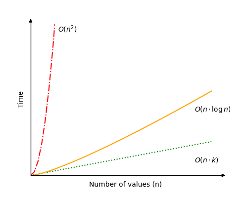
The time complexity for Radix Sort is: O(nk).
This means that Radix Sort depends both on the values that need to be sorted n, and the number of digits in the highest value k.
A best case scenario for Radix Sort is if there are lots of values to sort, but the values have few digits. For example if there are more than a million values to sort, and the highest value is 999, with just three digits. In such a case the time complexity O(nk) can be simplified to just O(n).
A worst case scenario for Radix Sort would be if there are as many digits in the highest value as there are values to sort. This is perhaps not a common scenario, but the time complexity would be O(n2) in this case.
The most average or common case is perhaps if the number of digits k is something like k(n) = logn. If so, Radix Sort gets time complexity O(nlogn). An example of such a case would be if there are 1000000 values to sort, and the values have 6 digits.
See different possible time complexities for Radix Sort in the image below.
Merge Sort
The Merge Sort algorithm is a divide-and-conquer algorithm that sorts an array by first breaking it down into smaller arrays, and then building the array back together the correct way so that it is sorted.
Divide: The algorithm starts with breaking up the array into smaller and smaller pieces until one such sub-array only consists of one element.
Conquer: The algorithm merges the small pieces of the array back together by putting the lowest values first, resulting in a sorted array.
The breaking down and building up of the array to sort the array is done recursively.
- How it works
- Divide the unsorted array into two sub-arrays, half the size of the original.
- Continue to divide the sub-arrays as long as the current piece of the array has more than one element.
- Merge two sub-arrays together by always putting the lowest value first.
- Keep merging until there are no sub-arrays left.
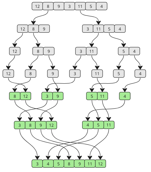
Take a look at the drawing below to see how Merge Sort works from a different perspective. As you can see, the array is split into smaller and smaller pieces until it is merged back together. And as the merging happens, values from each sub-array are compared so that the lowest value comes first.
- Implementation
To implement the Merge Sort algorithm we need:
- An array with values that needs to be sorted.
- A function that takes an array, splits it in two, and calls itself with each half of that array so that the arrays are split again and again recursively, until a sub-array only consist of one value.
- Another function that merges the sub-arrays back together in a sorted way.
The resulting code looks like this:
def mergeSort(arr):
    if len(arr) <= 1:
        return arr

    mid = len(arr) // 2
    leftHalf = arr[:mid]
    rightHalf = arr[mid:]

    sortedLeft = mergeSort(leftHalf)
    sortedRight = mergeSort(rightHalf)

    return merge(sortedLeft, sortedRight)

def merge(left, right):
    result = []
    i = j = 0

    while i < len(left) and j < len(right):
        if left[i] < right[j]:
            result.append(left[i])
            i += 1
        else:
            result.append(right[j])
            j += 1

    result.extend(left[i:])
    result.extend(right[j:])

    return result

unsortedArr = [3, 7, 6, -10, 15, 23.5, 55, -13]
sortedArr = mergeSort(unsortedArr)

print("Sorted array:", sortedArr)
- Time Complexity
The time complexity for Merge Sort is O(nlogn).
And the time complexity is pretty much the same for different kinds of arrays. The algorithm needs to split the array and merge it back together whether it is already sorted or completely shuffled.
Linear Search
The Linear Search algorithm searches through an array and returns the index of the value it searches for.
A big difference between sorting algorithms and searching algorithms is that sorting algorithms modify the array, but searching algorithms leave the array unchanged.
- How it works
- Go through the array value by value from the start.
- Compare each value to check if it is equal to the value we are looking for.
- If the value is found, return the index of that value.
- If the end of the array is reached and the value is not found, return -1 to indicate that the value was not found.
- Implementation
To implement the Linear Search algorithm we need:
- An array with values to search through.
- A target value to search for.
- A loop that goes through the array from start to end.
- An if-statement that compares the current value with the target value, and returns the current index if the target value is found.
- After the loop, return -1, because at this point we know the target value has not been found.
The resulting code for Linear Search looks like this:
def linearSearch(arr, targetVal):
    for i in range(len(arr)):
        if arr[i] == targetVal:
            return i
    return -1

arr = [3, 7, 2, 9, 5]
targetVal = 9

result = linearSearch(arr, targetVal)

if result != -1:
    print("Value", targetVal, "found at index", result)
else:
    print("Value", targetVal, "not found")
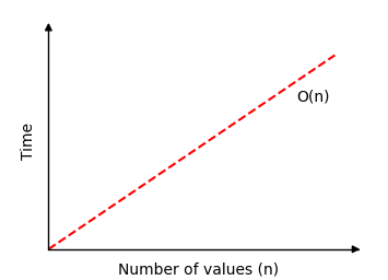
- Time Complexity
If Linear Search runs and finds the target value as the first array value in an array with n values, only one compare is needed.
But if Linear Search runs through the whole array of n values, without finding the target value, n compares are needed.
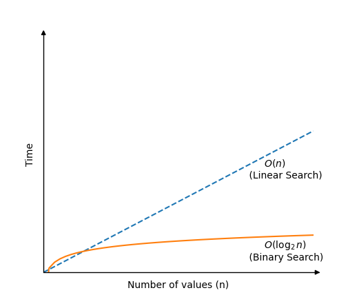
This means that time complexity for Linear Search is O(n).
If we draw how much time Linear Search needs to find a value in an array of n values, we get this graph:
Binary Search
The Binary Search algorithm searches through an array and returns the index of the value it searches for.
Binary Search is much faster than Linear Search, but requires a sorted array to work.
The Binary Search algorithm works by checking the value in the center of the array. If the target value is lower, the next value to check is in the center of the left half of the array. This way of searching means that the search area is always half of the previous search area, and this is why the Binary Search algorithm is so fast.
This process of halving the search area happens until the target value is found, or until the search area of the array is empty.
- How it works
- Check the value in the center of the array.
- If the target value is lower, search the left half of the array. If the target value is higher, search the right half.
- Continue step 1 and 2 for the new reduced part of the array until the target value is found or until the search area is empty.
- If the value is found, return the target value index. If the target value is not found, return -1.
- Implementation
To implement the Binary Search algorithm we need:
- An array with values to search through.
- A target value to search for.
- A loop that runs as long as left index is less than, or equal to, the right index.
- An if-statement that compares the middle value with the target value, and returns the index if the target value is found.
- An if-statement that checks if the target value is less than, or larger than, the middle value, and updates the "left" or "right" variables to narrow down the search area.
- After the loop, return -1, because at this point we know the target value has not been found.
The resulting code for Binary Search looks like this:
def binarySearch(arr, targetVal):
    left = 0
    right = len(arr) - 1

    while left <= right:
        mid = (left + right) // 2

        if arr[mid] == targetVal:
            return mid

        if arr[mid] < targetVal:
            left = mid + 1
        else:
            right = mid - 1

    return -1

myArray = [1, 3, 5, 7, 9, 11, 13, 15, 17, 19]
myTarget = 15

result = binarySearch(myArray, myTarget)

if result != -1:
    print("Value", myTarget, "found at index", result)
else:
    print("Target not found in array.")
- Time Complexity
Each time Binary Search checks a new value to see if it is the target value, the search area is halved.
This means that even in the worst case scenario where Binary Search cannot find the target value, it still only needs log2n comparisons to look through a sorted array of n values.
Time complexity for Binary Search is O(log2n).
Note: When writing time complexity using Big O notation we could also just have written O(logn), but O(log2n) reminds us that the array search area is halved for every new comparison, which is the basic concept of Binary Search, so we will just keep the base 2 indication in this case.
If we draw how much time Binary Search needs to find a value in an array of n values, compared to Linear Search, we get this graph:
Linked Lists
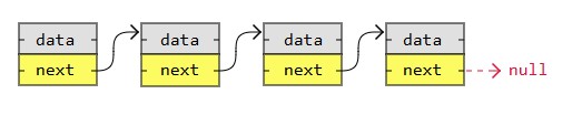
A Linked List is, as the word implies, a list where the nodes are linked together. Each node contains data and a pointer. The way they are linked together is that each node points to where in the memory the next node is placed.
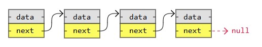
A linked list consists of nodes with some sort of data, and a pointer, or link, to the next node.
A big benefit with using linked lists is that nodes are stored wherever there is free space in memory, the nodes do not have to be stored contiguously right after each other like elements are stored in arrays. Another nice thing with linked lists is that when adding or removing nodes, the rest of the nodes in the list do not have to be shifted.
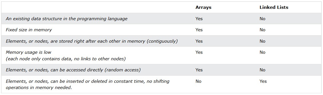
- Linked Lists vs. Arrays
The easiest way to understand linked lists is perhaps by comparing linked lists with arrays.
Linked lists consist of nodes, and is a linear data structure we make ourselves, unlike arrays which is an existing data structure in the programming language that we can use.
Nodes in a linked list store links to other nodes, but array elements do not need to store links to other elements.
The table below compares linked lists with arrays to give a better understanding of what linked lists are.
- Linked Lists in Memory
To explain what linked lists are, and how linked lists are different from arrays, we need to understand some basics about how computer memory works.
Computer memory is the storage your program uses when it is running. This is where your variables, arrays and linked lists are stored.
- Variables in Memory
Let's imagine that we want to store the integer "17" in a variable myNumber. For simplicity, let's assume the integer is stored as two bytes (16 bits), and the address in memory to myNumber is 0x7F25.
0x7F25 is actually the address to the first of the two bytes of memory where the myNumber integer value is stored. When the computer goes to 0x7F25 to read an integer value, it knows that it must read both the first and the second byte, since integers are two bytes on this specific computer.
The image below shows how the variable myNumber = 17 is stored in memory.
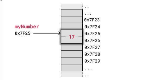
The example above shows how an integer value is stored on the simple, but popular, Arduino Uno microcontroller. This microcontroller has an 8 bit architecture with 16 bit address bus and uses two bytes for integers and two bytes for memory addresses. For comparison, personal computers and smart phones use 32 or 64 bits for integers and addresses, but the memory works basically in the same way.
- Arrays in Memory
To understand linked lists, it is useful to first know how arrays are stored in memory.
Elements in an array are stored contiguously in memory. That means that each element is stored right after the previous element.
The image below shows how an array of integers myArray = [3,5,13,2] is stored in memory. We use a simple kind of memory here with two bytes for each integer, like in the previous example, just to get the idea.
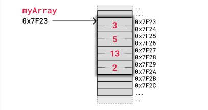
The computer has only got the address of the first byte of myArray, so to access the 3rd element with code myArray[2] the computer starts at 0x7F23 and jumps over the two first integers. The computer knows that an integer is stored in two bytes, so it jumps 2x2 bytes forward from 0x7F23 and reads value 13 starting at address 0x7F27.
When removing or inserting elements in an array, every element that comes after must be either shifted up to make place for the new element, or shifted down to take the removed element's place. Such shifting operations are time consuming and can cause problems in real-time systems for example.
The image below shows how elements are shifted when an array element is removed.

Manipulating arrays is also something you must think about if you are programming in C, where you have to explicitly move other elements when inserting or removing an element. In C this does not happen in the background.
In C you also need to make sure that you have allocated enough space for the array to start with, so that you can add more elements later.
- Linked Lists in Memory
Instead of storing a collection of data as an array, we can create a linked list.
Linked lists are used in many scenarios, like dynamic data storage, stack and queue implementation or graph representation, to mention some of them.
A linked list consists of nodes with some sort of data, and at least one pointer, or link, to other nodes.
A big benefit with using linked lists is that nodes are stored wherever there is free space in memory, the nodes do not have to be stored contiguously right after each other like elements are stored in arrays. Another nice thing with linked lists is that when adding or removing nodes, the rest of the nodes in the list do not have to be shifted.
The image below shows how a linked list can be stored in memory. The linked list has four nodes with values 3, 5, 13 and 2, and each node has a pointer to the next node in the list.
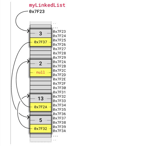
Each node takes up four bytes. Two bytes are used to store an integer value, and two bytes are used to store the address to the next node in the list. As mentioned before, how many bytes that are needed to store integers and addresses depend on the architecture of the computer. This example, like the previous array example, fits with a simple 8-bit microcontroller architecture.
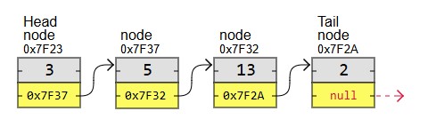
The first node in a linked list is called the "Head", and the last node is called the "Tail".
Unlike with arrays, the nodes in a linked list are not placed right after each other in memory. This means that when inserting or removing a node, shifting of other nodes is not necessary, so that is a good thing.
Something not so good with linked lists is that we cannot access a node directly like we can with an array by just writing myArray[5] for example. To get to node number 5 in a linked list, we must start with the first node called "head", use that node's pointer to get to the next node, and do so while keeping track of the number of nodes we have visited until we reach node number 5.
Learning about linked lists helps us to better understand concepts like memory allocation and pointers.
Linked lists are also important to understand before learning about more complex data structures such as trees and graphs, that can be implemented using linked lists.
- Memory in Modern Computers
So far on this page we have used the memory in an 8 bit microcontroller as an example to keep it simple and easier to understand.
Memory in modern computers work in the same way in principle as memory in an 8 bit microcontroller, but more memory is used to store integers, and more memory is used to store memory addresses.
The code below gives us the size of an integer and the size of a memory address on the server we are running these examples on.
#include <stdio.h>

int main() {
    int myVal = 13;

    printf("Value of integer 'myVal': %d\n", myVal);
    printf("Size of integer 'myVal': %lu bytes\n", sizeof(myVal)); // 4 bytes
    printf("Address to 'myVal': %p\n", &myVal);
    printf("Size of the address to 'myVal': %lu bytes\n", sizeof(&myVal)); // 8 bytes

    return 0;
}
- Linked List Implementation in C
Let's implement this linked list in C to see a concrete example of how linked lists are stored in memory.
In the code below, after including the libraries, we create a node struct which is like a class that represents what a node is: the node contains data and a pointer to the next node.
The createNode() function allocates memory for a new node, fills in the data part of the node with an integer given as an argument to the function, and returns the pointer (memory address) to the new node.
The printList() function is just for going through the linked list and printing each node's value.
Inside the main() function, four nodes are created, linked together, printed, and then the memory is freed. It is good practice to free memory after we are done using it to avoid memory leaks. Memory leak is when memory is not freed after use, gradually taking up more and more memory.
#include <stdio.h>
#include <stdlib.h>

// Define the Node struct
typedef struct Node {
    int data;
    struct Node* next;
} Node;

// Create a new node
Node* createNode(int data) {
    Node* newNode = (Node*)malloc(sizeof(Node));

    if (!newNode) {
        printf("Memory allocation failed!\n");
        exit(1);
    }

    newNode->data = data;
    newNode->next = NULL;

    return newNode;
}

// Print the linked list
void printList(Node* node) {
    while (node) {
        printf("%d -> ", node->data);
        node = node->next;
    }

    printf("null\n");
}

int main() {
    // Explicitly creating and connecting nodes
    Node* node1 = createNode(3);
    Node* node2 = createNode(5);
    Node* node3 = createNode(13);
    Node* node4 = createNode(2);

    node1->next = node2;
    node2->next = node3;
    node3->next = node4;

    printList(node1);

    // Free the memory
    free(node1);
    free(node2);
    free(node3);
    free(node4);

    return 0;
}
To print the linked list in the code above, the printList() function goes from one node to the next using the "next" pointers, and that is called "traversing" or "traversal" of the linked list.
- Linked Lists Types
There are three basic forms of linked lists:
- Singly linked lists
- Doubly linked lists
- Circular linked lists
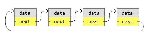
A singly linked list is the simplest kind of linked lists. It takes up less space in memory because each node has only one address to the next node, like in the image below.
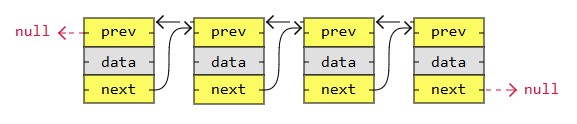
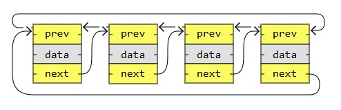
A doubly linked list has nodes with addresses to both the previous and the next node, like in the image below, and therefore takes up more memory. But doubly linked lists are good if you want to be able to move both up and down in the list.
A circular linked list is like a singly or doubly linked list with the first node, the "head", and the last node, the "tail", connected.
In singly or doubly linked lists, we can find the start and end of a list by just checking if the links are null. But for circular linked lists, more complex code is needed to explicitly check for start and end nodes in certain applications.
Circular linked lists are good for lists you need to cycle through continuously.
The image below is an example of a singly circular linked list:
The image below is an example of a doubly circular linked list:
Note: What kind of linked list you need depends on the problem you are trying to solve.
- Implementations
Below are basic implementations of:
- Singly linked list
- Doubly linked list
- Circular singly linked list
- Circular doubly linked list
# Singly Linked List Implementation
class Node:
    def __init__(self, data):
        self.data = data
        self.next = None

node1 = Node(3)
node2 = Node(5)
node3 = Node(13)
node4 = Node(2)

node1.next = node2
node2.next = node3
node3.next = node4

currentNode = node1
while currentNode:
    print(currentNode.data, end=" -> ")
    currentNode = currentNode.next
print("null")
# Doubly Linked List Implementation
class Node:
    def __init__(self, data):
        self.data = data
        self.next = None
        self.prev = None

node1 = Node(3)
node2 = Node(5)
node3 = Node(13)
node4 = Node(2)

node1.next = node2

node2.prev = node1
node2.next = node3

node3.prev = node2
node3.next = node4

node4.prev = node3

print("\nTraversing forward:")
currentNode = node1
while currentNode:
    print(currentNode.data, end=" -> ")
    currentNode = currentNode.next
print("null")

print("\nTraversing backward:")
currentNode = node4
while currentNode:
    print(currentNode.data, end=" -> ")
    currentNode = currentNode.prev
print("null")
# Circular Singly Linked List Implementation
class Node:
    def __init__(self, data):
        self.data = data
        self.next = None

node1 = Node(3)
node2 = Node(5)
node3 = Node(13)
node4 = Node(2)

node1.next = node2
node2.next = node3
node3.next = node4
node4.next = node1 # Circular link

currentNode = node1
startNode = node1
print(currentNode.data, end=" -> ")
currentNode = currentNode.next

while currentNode != startNode:
    print(currentNode.data, end=" -> ")
    currentNode = currentNode.next

print("...") # Indicating the list loops back
# Circular Doubly Linked List Implementation
class Node:
    def __init__(self, data):
        self.data = data
        self.next = None
        self.prev = None

node1 = Node(3)
node2 = Node(5)
node3 = Node(13)
node4 = Node(2)

node1.next = node2
node1.prev = node4  # Circular link

node2.prev = node1
node2.next = node3

node3.prev = node2
node3.next = node4

node4.prev = node3
node4.next = node1  # Circular link

print("\nTraversing forward:")
currentNode = node1
startNode = node1
print(currentNode.data, end=" -> ")
currentNode = currentNode.next

while currentNode != startNode:
    print(currentNode.data, end=" -> ")
    currentNode = currentNode.next
print("...")  # Indicating it's circular

print("\nTraversing backward:")
currentNode = node4
startNode = node4
print(currentNode.data, end=" -> ")
currentNode = currentNode.prev

while currentNode != startNode:
    print(currentNode.data, end=" -> ")
    currentNode = currentNode.prev
print("...")  # Indicating it's circular
- Linked List Operations
Basic things we can do with linked lists are:
- Traversal
- Remove a node
- Insert a node
- Sort
- Traversal of a Linked List
Traversing a linked list means to go through the linked list by following the links from one node to the next.
Traversal of linked lists is typically done to search for a specific node, and read or modify the node's content, remove the node, or insert a node right before or after that node.
To traverse a singly linked list, we start with the first node in the list, the head node, and follow that node's next link, and the next node's next link and so on, until the next address is null.
The code below prints out the node values as it traverses along the linked list.
class Node:
    def __init__(self, data):
        self.data = data
        self.next = None

def traverseAndPrint(head):
    currentNode = head
    while currentNode:
        print(currentNode.data, end=" -> ")
        currentNode = currentNode.next
    print("null")

node1 = Node(7)
node2 = Node(11)
node3 = Node(3)
node4 = Node(2)
node5 = Node(9)

node1.next = node2
node2.next = node3
node3.next = node4
node4.next = node5

traverseAndPrint(node1)
- Find The Lowest Value in a Linked List
Let's find the lowest value in a singly linked list by traversing it and checking each value.
Finding the lowest value in a linked list is very similar to how we found the lowest value in an array, except that we need to follow the next link to get to the next node.
To find the lowest value we need to traverse the list like in the previous code. But in addition to traversing the list, we must also update the current lowest value when we find a node with a lower value.
In the code below, the algorithm to find the lowest value is moved into a function called findLowestValue.
class Node:
    def __init__(self, data):
        self.data = data
        self.next = None

def findLowestValue(head):
    minValue = head.data
    currentNode = head.next
    while currentNode:
        if currentNode.data < minValue:
            minValue = currentNode.data
        currentNode = currentNode.next
    return minValue

node1 = Node(7)
node2 = Node(11)
node3 = Node(3)
node4 = Node(2)
node5 = Node(9)

node1.next = node2
node2.next = node3
node3.next = node4
node4.next = node5

print("The lowest value in the linked list is:", findLowestValue(node1))
- Delete a Node in a Linked List
In this case we have the link (or pointer or address) to a node that we want to delete.
It is important to connect the nodes on each side of the node before deleting it, so that the linked list is not broken.
So before deleting the node, we need to get the next pointer from the previous node, and connect the previous node to the new next node before deleting the node in between.
Also, it is a good idea to first connect next pointer to the node after the node we want to delete, before we delete it. This is to avoid a 'dangling' pointer, a pointer that points to nothing, even if it is just for a brief moment.
In the code below, the algorithm to delete a node is moved into a function called deleteSpecificNode.
class Node:
    def __init__(self, data):
        self.data = data
        self.next = None

def traverseAndPrint(head):
    currentNode = head
    while currentNode:
        print(currentNode.data, end=" -> ")
        currentNode = currentNode.next
    print("null")

def deleteSpecificNode(head, nodeToDelete):
    if head == nodeToDelete:
        return head.next

    currentNode = head
    while currentNode.next and currentNode.next != nodeToDelete:
        currentNode = currentNode.next

    if currentNode.next is None:
        return head

    currentNode.next = currentNode.next.next

    return head

node1 = Node(7)
node2 = Node(11)
node3 = Node(3)
node4 = Node(2)
node5 = Node(9)

node1.next = node2
node2.next = node3
node3.next = node4
node4.next = node5

print("Before deletion:")
traverseAndPrint(node1)

# Delete node4
node1 = deleteSpecificNode(node1, node4)

print("\nAfter deletion:")
traverseAndPrint(node1)
In the deleteSpecificNode function above, the return value is the new head of the linked list. So for example, if the node to be deleted is the first node, the new head returned will be the next node.
- Insert a Node in a Linked List
Inserting a node into a linked list is very similar to deleting a node, because in both cases we need to take care of the next pointers to make sure we do not break the linked list.
To insert a node in a linked list we first need to create the node, and then at the position where we insert it, we need to adjust the pointers so that the previous node points to the new node, and the new node points to the correct next node.
- New node is created
- Node 1 is linked to new node
- New node is linked to next node
class Node:
    def __init__(self, data):
        self.data = data
        self.next = None

def traverseAndPrint(head):
    currentNode = head
    while currentNode:
        print(currentNode.data, end=" -> ")
        currentNode = currentNode.next
    print("null")

def insertNodeAtPosition(head, newNode, position):
    if position == 1:
        newNode.next = head
        return newNode

    currentNode = head
    for _ in range(position - 2):
        if currentNode is None:
            break
        currentNode = currentNode.next

    newNode.next = currentNode.next
    currentNode.next = newNode
    return head

node1 = Node(7)
node2 = Node(3)
node3 = Node(2)
node4 = Node(9)

node1.next = node2
node2.next = node3
node3.next = node4

print("Original list:")
traverseAndPrint(node1)

# Insert a new node with value 97 at position 2
newNode = Node(97)
node1 = insertNodeAtPosition(node1, newNode, 2)

print("\nAfter insertion:")
traverseAndPrint(node1)
- Time Complexity of Linked Lists Operations
We have only covered three basic linked list operations above: traversal (or search), node deletion, and node insertion.
There are a lot of other operations that could be done with linked lists, like sorting for example.
Here we discuss time complexity of linked list operations, and compare these with the time complexity of the array algorithms.
Remember that time complexity just says something about the approximate number of operations needed by the algorithm based on a large set of data n, and does not tell us the exact time a specific implementation of an algorithm takes.
This means that even though linear search is said to have the same time complexity for arrays as for linked list: O(n), it does not mean they take the same amount of time. The exact time it takes for an algorithm to run depends on programming language, computer hardware, differences in time needed for operations on arrays vs linked lists, and many other things as well.
Linear search for linked lists works the same as for arrays. A list of unsorted values are traversed from the head node until the node with the specific value is found. Time complexity is O(n).
Binary search is not possible for linked lists because the algorithm is based on jumping directly to different array elements, and that is not possible with linked lists.
Sorting algorithms have the same time complexities as for arrays. But remember, sorting algorithms that are based on directly accessing an array element based on an index, do not work on linked lists.
Stacks
A stack is a data structure that can hold many elements.
Think of a stack like a pile of pancakes.
In a pile of pancakes, the pancakes are both added and removed from the top. So when removing a pancake, it will always be the last pancake you added. This way of organizing elements is called LIFO: Last In First Out.
Basic operations we can do on a stack are:
- Push: Adds a new element on the stack.
- Pop: Removes and returns the top element from the stack.
- Peek: Returns the top element on the stack.
- isEmpty: Checks if the stack is empty.
- Size: Finds the number of elements in the stack.
Stacks can be implemented by using arrays or linked lists.
Stacks can be used to implement undo mechanisms, to revert to previous states, to create algorithms for depth-first search in graphs, or for backtracking.
Stacks are often mentioned together with Queues, which is a similar data structure.
- Implementation using Arrays
Reasons to implement stacks using arrays:
- Memory Efficient: Array elements do not hold the next elements address like linked list nodes do.
- Easier to implement and understand: Using arrays to implement stacks require less code than using linked lists, and for this reason it is typically easier to understand as well.
A reason for not using arrays to implement stacks:
- Fixed size: An array occupies a fixed part of the memory. This means that it could take up more memory than needed, or if the array fills up, it cannot hold more elements.
Note: When using arrays in Python for this tutorial, we are really using the Python 'list' data type, but for the scope of this tutorial the 'list' data type can be used in the same way as an array.
Since Python lists has good support for functionality needed to implement stacks, we start with creating a stack and do stack operations with just a few lines like this:
stack = []

# Push
stack.append('A')
stack.append('B')
stack.append('C')
print("Stack: ", stack)

# Pop
element = stack.pop()
print("Pop: ", element)

# Peek
topElement = stack[-1]
print("Peek: ", topElement)

# isEmpty
isEmpty = not bool(stack)
print("isEmpty: ", isEmpty)

# Size
print("Size: ", len(stack))
But to explicitly create a data structure for stacks, with basic operations, we should create a stack class instead. This way of creating stacks in Python is also more similar to how stacks can be created in other programming languages like C and Java.
class Stack:
    def __init__(self):
        self.stack = []

    def push(self, element):
        self.stack.append(element)

    def pop(self):
        if self.isEmpty():
            return "Stack is empty"
        return self.stack.pop()

    def peek(self):
        if self.isEmpty():
            return "Stack is empty"
        return self.stack[-1]

    def isEmpty(self):
        return len(self.stack) == 0

    def size(self):
        return len(self.stack)

# Create a stack
myStack = Stack()

myStack.push('A')
myStack.push('B')
myStack.push('C')

print("Stack: ", myStack.stack)
print("Pop: ", myStack.pop())
print("Peek: ", myStack.peek())
print("isEmpty: ", myStack.isEmpty())
print("Size: ", myStack.size())
- Implementation using Linked Lists
A reason for using linked lists to implement stacks:
- Dynamic size: The stack can grow and shrink dynamically, unlike with arrays.
Reasons for not using linked lists to implement stacks:
- Extra memory: Each stack element must contain the address to the next element (the next linked list node).
- Readability: The code might be harder to read and write for some because it is longer and more complex.
This is how a stack can be implemented using a linked list.
class Node:
    def __init__(self, value):
        self.value = value
        self.next = None

class Stack:
    def __init__(self):
        self.head = None
        self.size = 0

    def push(self, value):
        new_node = Node(value)
        if self.head:
            new_node.next = self.head
        self.head = new_node
        self.size += 1

    def pop(self):
        if self.isEmpty():
            return "Stack is empty"
        popped_node = self.head
        self.head = self.head.next
        self.size -= 1
        return popped_node.value

    def peek(self):
        if self.isEmpty():
            return "Stack is empty"
        return self.head.value

    def isEmpty(self):
        return self.size == 0

    def stackSize(self):
        return self.size

# Usage
myStack = Stack()
myStack.push('A')
myStack.push('B')
myStack.push('C')

print("Pop: ", myStack.pop())
print("Peek: ", myStack.peek())
print("isEmpty: ", myStack.isEmpty())
print("Size: ", myStack.stackSize())
Queues
A queue is a data structure that can hold many elements.
Think of a queue as people standing in line in a supermarket.
The first person to stand in line is also the first who can pay and leave the supermarket. This way of organizing elements is called FIFO: First In First Out.
Basic operations we can do on a queue are:
- Enqueue: Adds a new element to the queue.
- Dequeue: Removes and returns the first (front) element from the queue.
- Peek: Returns the first element in the queue.
- isEmpty: Checks if the queue is empty.
- Size: Finds the number of elements in the queue.
Queues can be implemented by using arrays or linked lists.
Queues can be used to implement job scheduling for an office printer, order processing for e-tickets, or to create algorithms for breadth-first search in graphs.
Queues are often mentioned together with Stacks, which is a similar data structure.
- Implementation using Arrays
Reasons to implement queues using arrays:
- Memory Efficient: Array elements do not hold the next elements address like linked list nodes do.
- Easier to implement and understand: Using arrays to implement queues require less code than using linked lists, and for this reason it is typically easier to understand as well.
Reasons for not using arrays to implement queues:
- Fixed size: An array occupies a fixed part of the memory. This means that it could take up more memory than needed, or if the array fills up, it cannot hold more elements. And resizing an array can be costly.
- Shifting cost: Dequeue causes the first element in a queue to be removed, and the other elements must be shifted to take the removed elements' place. This is inefficient and can cause problems, especially if the queue is long.
- Alternatives: Some programming languages have built-in data structures optimized for queue operations that are better than using arrays.
Since Python lists has good support for functionality needed to implement queues, we start with creating a queue and do queue operations with just a few lines:
queue = []

# Enqueue
queue.append('A')
queue.append('B')
queue.append('C')
print("Queue: ", queue)

# Dequeue
element = queue.pop(0)
print("Dequeue: ", element)

# Peek
frontElement = queue[0]
print("Peek: ", frontElement)

# isEmpty
isEmpty = not bool(queue)
print("isEmpty: ", isEmpty)

# Size
print("Size: ", len(queue))
But to explicitly create a data structure for queues, with basic operations, we should create a queue class instead. This way of creating queues in Python is also more similar to how queues can be created in other programming languages like C and Java.
class Queue:
    def __init__(self):
        self.queue = []

    def enqueue(self, element):
        self.queue.append(element)

    def dequeue(self):
        if self.isEmpty():
            return "Queue is empty"
        return self.queue.pop(0)

    def peek(self):
        if self.isEmpty():
            return "Queue is empty"
        return self.queue[0]

    def isEmpty(self):
        return len(self.queue) == 0

    def size(self):
        return len(self.queue)

# Create a queue
myQueue = Queue()

myQueue.enqueue('A')
myQueue.enqueue('B')
myQueue.enqueue('C')

print("Queue: ", myQueue.queue)
print("Dequeue: ", myQueue.dequeue())
print("Peek: ", myQueue.peek())
print("isEmpty: ", myQueue.isEmpty())
print("Size: ", myQueue.size())
- Implementation using Linked Lists
Reasons for using linked lists to implement queues:
- Dynamic size: The queue can grow and shrink dynamically, unlike with arrays.
- No shifting: The front element of the queue can be removed (enqueue) without having to shift other elements in the memory.
Reasons for not using linked lists to implement queues:
- Extra memory: Each queue element must contain the address to the next element (the next linked list node).
- Readability: The code might be harder to read and write for some because it is longer and more complex.
This is how a queue can be implemented using a linked list.
class Node:
    def __init__(self, data):
        self.data = data
        self.next = None

class Queue:
    def __init__(self):
        self.front = None
        self.rear = None
        self.length = 0

    def enqueue(self, element):
        new_node = Node(element)
        if self.rear is None:
            self.front = self.rear = new_node
            self.length += 1
            return
        self.rear.next = new_node
        self.rear = new_node
        self.length += 1

    def dequeue(self):
        if self.isEmpty():
            return "Queue is empty"
        temp = self.front
        self.front = temp.next
        self.length -= 1
        if self.front is None:
            self.rear = None
        return temp.data

    def peek(self):
        if self.isEmpty():
            return "Queue is empty"
        return self.front.data

    def isEmpty(self):
        return self.length == 0

    def size(self):
        return self.length

    def printQueue(self):
        temp = self.front
        while temp:
            print(temp.data, end=" ")
            temp = temp.next
        print()

# Create a queue
myQueue = Queue()

myQueue.enqueue('A')
myQueue.enqueue('B')
myQueue.enqueue('C')
print("Queue: ", end="")
myQueue.printQueue()

print("Dequeue: ", myQueue.dequeue())
print("Peek: ", myQueue.peek())
print("isEmpty: ", myQueue.isEmpty())
print("Size: ", myQueue.size())
Hash Tables
A Hash Table is a data structure designed to be fast to work with.
The reason Hash Tables are sometimes preferred instead of arrays or linked lists is because searching for, adding, and deleting data can be done really quickly, even for large amounts of data.
In a Linked List, finding a person "Bob" takes time because we would have to go from one node to the next, checking each node, until the node with "Bob" is found.
And finding "Bob" in an Array could be fast if we knew the index, but when we only know the name "Bob", we need to compare each element (like with Linked Lists), and that takes time.
With a Hash Table however, finding "Bob" is done really fast because there is a way to go directly to where "Bob" is stored, using something called a hash function.
- Building A Hash Table from Scratch
To get the idea of what a Hash Table is, let's try to build one from scratch, to store unique first names inside it.
We will build the Hash Set in 5 steps:
- Starting with an array.
- Storing names using a hash function.
- Looking up an element using a hash function.
- Handling collisions.
- The basic Hash Set code example.
# Step 1: Starting with an array
Using an array, we could store names like this:
my_array = ['Pete', 'Jones', 'Lisa', 'Bob', 'Siri']
To find "Bob" in this array, we need to compare each name, element by element, until we find "Bob".
If the array was sorted alphabetically, we could use Binary Search to find a name quickly, but inserting or deleting names in the array would mean a big operation of shifting elements in memory.
To make interacting with the list of names really fast, let's use a Hash Table for this instead, or a Hash Set, which is a simplified version of a Hash Table.
To keep it simple, let's assume there is at most 10 names in the list, so the array must be a fixed size of 10 elements. When talking about Hash Tables, each of these elements is called a bucket.
my_hash_set = [None,None,None,None,None,None,None,None,None,None]
# Step 2: Storing names using a hash function
Now comes the special way we interact with the Hash Set we are making.
We want to store a name directly into its right place in the array, and this is where the hash function comes in.
A hash function can be made in many ways, it is up to the creator of the Hash Table. A common way is to find a way to convert the value into a number that equals one of the Hash Set's index numbers, in this case a number from 0 to 9. In our example we will use the Unicode number of each character, summarize them and do a modulo 10 operation to get index numbers 0-9.
def hash_function(value):
    sum_of_chars = 0
    for char in value:
        sum_of_chars += ord(char)

    return sum_of_chars % 10

print("'Bob' has hash code:", hash_function('Bob'))
The character "B" has Unicode code point 66, "o" has 111, and "b" has 98. Adding those together we get 275. Modulo 10 of 275 is 5, so "Bob" should be stored as an array element at index 5.
The number returned by the hash function is called the hash code.
Unicode number: Everything in our computers are stored as numbers, and the Unicode code point is a unique number that exist for every character. For example, the character A has Unicode number (also called Unicode code point) 65. Modulo: A mathematical operation, written as % in most programming languages (or mod in mathematics). A modulo operation divides a number with another number, and gives us the resulting remainder. So for example, 7 % 3 will give us the remainder 1. (Dividing 7 apples between 3 people, means that each person gets 2 apples, with 1 apple to spare.)
After storing "Bob" where the hash code tells us (index 5), our array now looks like this:
my_hash_set = [None,None,None,None,None,'Bob',None,None,None,None]
We can use the hash function to find out where to store the other names "Pete", "Jones", "Lisa", and "Siri" as well.
After using the hash function to store those names in the correct position, our array looks like this:
my_hash_set = [None,'Jones',None,'Lisa',None,'Bob',None,'Siri','Pete',None]
# Step 3: Looking up a name using a hash function
We have now established a super basic Hash Set, because we do not have to check the array element by element anymore to find out if "Pete" is in there, we can just use the hash function to go straight to the right element!
To find out if "Pete" is stored in the array, we give the name "Pete" to our hash function, we get back hash code 8, we go directly to the element at index 8, and there he is. We found "Pete" without checking any other elements.
my_hash_set = [None,'Jones',None,'Lisa',None,'Bob',None,'Siri','Pete',None]

def hash_function(value):
    sum_of_chars = 0
    for char in value:
        sum_of_chars += ord(char)

    return sum_of_chars % 10

def contains(name):
    index = hash_function(name)
    return my_hash_set[index] == name

print("'Pete' is in the Hash Set:", contains('Pete'))
When deleting a name from our Hash Set, we can also use the hash function to go straight to where the name is, and set that element value to None.
# Step 4: Handling collisions
Let's also add "Stuart" to our Hash Set.
We give "Stuart" to our hash function, and we get the hash code 3, meaning "Stuart" should be stored at index 3.
Trying to store "Stuart" creates what is called a collision, because "Lisa" is already stored at index 3.
To fix the collision, we can make room for more elements in the same bucket, and solving the collision problem in this way is called chaining. We can give room for more elements in the same bucket by implementing each bucket as a linked list, or as an array.
After implementing each bucket as an array, to give room for potentially more than one name in each bucket, "Stuart" can also be stored at index 3, and our Hash Set now looks like this:
my_hash_set = [
    [None],
    ['Jones'],
    [None],
    ['Lisa', 'Stuart'],
    [None],
    ['Bob'],
    [None],
    ['Siri'],
    ['Pete'],
    [None]
]
Searching for "Stuart" in our Hash Set now means that using the hash function we end up directly in bucket 3, but then be must first check "Lisa" in that bucket, before we find "Stuart" as the second element in bucket 3.
# Step 5: Hash Set code example
To complete our very basic Hash Set code, let's have functions for adding and searching for names in the Hash Set, which is now a two dimensional array.
my_hash_set = [
    [None],
    ['Jones'],
    [None],
    ['Lisa'],
    [None],
    ['Bob'],
    [None],
    ['Siri'],
    ['Pete'],
    [None]
]

def hash_function(value):
    return sum(ord(char) for char in value) % 10

def add(value):
    index = hash_function(value)
    bucket = my_hash_set[index]
    if value not in bucket:
        bucket.append(value)

def contains(value):
    index = hash_function(value)
    bucket = my_hash_set[index]
    return value in bucket

add('Stuart')

print(my_hash_set)
print('Contains Stuart:', contains('Stuart'))
Hash Sets
A Hash Set is a form of Hash Table data structure that usually holds a large number of elements.
Using a Hash Set we can search, add, and remove elements really fast.
Hash Sets are used for lookup, to check if an element is part of a set.
A Hash Set stores unique elements in buckets according to the element's hash code.
- Hash code: A number generated from an element's unique value (key), to determine what bucket that Hash Set element belongs to.
- Unique elements: A Hash Set cannot have more than one element with the same value.
- Bucket: A Hash Set consists of many such buckets, or containers, to store elements. If two elements have the same hash code, they belong to the same bucket. The buckets are therefore often implemented as arrays or linked lists, because a bucket needs to be able to hold more than one element.
A hash code is generated by a hash function.
The Hash Code gives us instant access as long as there is just one name in the corresponding bucket.
To keep Hash Sets fast, it is therefore important to have a hash function that will distribute the elements evenly between the buckets, and to have around as many buckets as Hash Set elements.
Having a lot more buckets than Hash Set elements is a waste of memory, and having a lot less buckets than Hash Set elements is a waste of time.
- Hash Set Implementation
Hash Sets in Python are typically done by using Python's own set data type, but to get a better understanding of how Hash Sets work we will not use that here.
To implement a Hash Set in Python we create a class SimpleHashSet.
Inside the SimpleHashSet class we have a method __init__ to initialize the Hash Set, a method hash_function for the hash function, and methods for the basic Hash Set operations: add, contains, and remove.
We also create a method print_set to better see how the Hash Set looks like.
class SimpleHashSet:
    def __init__(self, size=100):
        self.size = size
        self.buckets = [[] for _ in range(size)]  # A list of buckets, each is a list (to handle collisions)

    def hash_function(self, value):
        # Simple hash function: sum of character codes modulo the number of buckets
        return sum(ord(char) for char in value) % self.size

    def add(self, value):
        # Add a value if it's not already present
        index = self.hash_function(value)
        bucket = self.buckets[index]
        if value not in bucket:
            bucket.append(value)

    def contains(self, value):
        # Check if a value exists in the set
        index = self.hash_function(value)
        bucket = self.buckets[index]
        return value in bucket

    def remove(self, value):
        # Remove a value
        index = self.hash_function(value)
        bucket = self.buckets[index]
        if value in bucket:
            bucket.remove(value)

    def print_set(self):
        # Print all elements in the hash set
        print("Hash Set Contents:")
        for index, bucket in enumerate(self.buckets):
            print(f"Bucket {index}: {bucket}")

# Creating the Hash Set from the simulation
hash_set = SimpleHashSet(size=10)

hash_set.add("Charlotte")
hash_set.add("Thomas")
hash_set.add("Jens")
hash_set.add("Peter")
hash_set.add("Lisa")
hash_set.add("Adele")
hash_set.add("Michaela")
hash_set.add("Bob")

hash_set.print_set()

print("\n'Peter' is in the set:",hash_set.contains('Peter'))
print("Removing 'Peter'")
hash_set.remove('Peter')
print("'Peter' is in the set:",hash_set.contains('Peter'))
print("'Adele' has hash code:",hash_set.hash_function('Adele'))
Hash Maps
A Hash Map is a form of Hash Table data structure that usually holds a large number of entries.
Using a Hash Map we can search, add, modify, and remove entries really fast.
Hash Maps are used to find detailed information about something.
- Entry: Consists of a key and a value, forming a key-value pair.
- Key: Unique for each entry in the Hash Map. Used to generate a hash code determining the entry's bucket in the Hash Map. This ensures that every entry can be efficiently located.
- Hash Code: A number generated from an entry's key, to determine what bucket that Hash Map entry belongs to.
- Bucket: A Hash Map consists of many such buckets, or containers, to store entries.
- Value: Can be nearly any kind of information, like name, birth date, and address of a person. The value can be many different kinds of information combined.
- Hash Map Implementation
Hash Maps in Python are typically done by using Python's own dictionary data type, but to get a better understanding of how Hash Maps work we will not use that here.
To implement a Hash Map in Python we create a class SimpleHashMap.
Inside the SimpleHashMap class we have a method __init__ to initialize the Hash Map, a method hash_function for the hash function, and methods for the basic Hash Map operations: put, get, and remove.
We also create a method print_map to better see how the Hash Map looks like.
class SimpleHashMap:
    def __init__(self, size=100):
        self.size = size
        self.buckets = [[] for _ in range(size)]  # A list of buckets, each is a list (to handle collisions)

    def hash_function(self, key):
        # Sum only the numerical values of the key, ignoring non-numeric characters
        numeric_sum = sum(int(char) for char in key if char.isdigit())
        return numeric_sum % 10  # Perform modulo 10 on the sum

    def put(self, key, value):
        # Add or update a key-value pair
        index = self.hash_function(key)
        bucket = self.buckets[index]
        for i, (k, v) in enumerate(bucket):
            if k == key:
                bucket[i] = (key, value)  # Update existing key
                return
        bucket.append((key, value))  # Add new key-value pair if not found

    def get(self, key):
        # Retrieve a value by key
        index = self.hash_function(key)
        bucket = self.buckets[index]
        for k, v in bucket:
            if k == key:
                return v
        return None  # Key not found

    def remove(self, key):
        # Remove a key-value pair
        index = self.hash_function(key)
        bucket = self.buckets[index]
        for i, (k, v) in enumerate(bucket):
            if k == key:
                del bucket[i]  # Remove the key-value pair
                return

    def print_map(self):
        # Print all key-value pairs in the hash map
        print("Hash Map Contents:")
        for index, bucket in enumerate(self.buckets):
            print(f"Bucket {index}: {bucket}")

# Creating the Hash Map from the simulation
hash_map = SimpleHashMap(size=10)

# Adding some entries
hash_map.put("123-4567", "Charlotte")
hash_map.put("123-4568", "Thomas")
hash_map.put("123-4569", "Jens")
hash_map.put("123-4570", "Peter")
hash_map.put("123-4571", "Lisa")
hash_map.put("123-4672", "Adele")
hash_map.put("123-4573", "Michaela")
hash_map.put("123-6574", "Bob")

hash_map.print_map()

print("\nName associated with '123-4570':", hash_map.get("123-4570"))

print("Updating the name for '123-4570' to 'James'")
hash_map.put("123-4570","James")

print("Name associated with '123-4570':", hash_map.get("123-4570"))
Trees
The Tree data structure is similar to Linked Lists in that each node contains data and can be linked to other nodes.
We have previously covered data structures like Arrays, Linked Lists, Stacks, and Queues. These are all linear structures, which means that each element follows directly after another in a sequence. Trees however, are different. In a Tree, a single element can have multiple 'next' elements, allowing the data structure to branch out in various directions.
The data structure is called a "tree" because it looks like a tree, only upside down, just like in the image below.
The Tree data structure can be useful in many cases:
- Hierarchical Data: File systems, organizational models, etc.
- Databases: Used for quick data retrieval.
- Routing Tables: Used for routing data in network algorithms.
- Sorting/Searching: Used for sorting data and searching for data.
- Priority Queues: Priority queue data structures are commonly implemented using trees, such as binary heaps.
- Tree Terminology and Rules
- The first node in a tree is called the root node.
- A link connecting one node to another is called an edge.
- A parent node has links to its child nodes. Another word for a parent node is internal node.
- A node can have zero, one, or many child nodes.
- A node can only have one parent node.
- Nodes without links to other child nodes are called leaves, or leaf nodes.
- The tree height is the maximum number of edges from the root node to a leaf node. The height of the tree above is 2.
- The height of a node is the maximum number of edges between the node and a leaf node.
- The tree size is the number of nodes in the tree.
- Types of Trees
Trees are a fundamental data structure in computer science, used to represent hierarchical relationships.
- Binary Trees: Each node has up to two children, the left child node and the right child node. This structure is the foundation for more complex tree types like Binay Search Trees and AVL Trees.
- Binary Search Trees (BSTs): A type of Binary Tree where for each node, the left child node has a lower value, and the right child node has a higher value.
- AVL Trees: A type of Binary Search Tree that self-balances so that for every node, the difference in height between the left and right subtrees is at most one. This balance is maintained through rotations when nodes are inserted or deleted.
Binary Trees
A Binary Tree is a type of tree data structure where each node can have a maximum of two child nodes, a left child node and a right child node.
This restriction, that a node can have a maximum of two child nodes, gives us many benefits:
- Algorithms like traversing, searching, insertion and deletion become easier to understand, to implement, and run faster.
- Keeping data sorted in a Binary Search Tree (BST) makes searching very efficient.
- Balancing trees is easier to do with a limited number of child nodes, using an AVL Binary Tree for example.
- Binary Trees can be represented as arrays, making the tree more memory efficient.
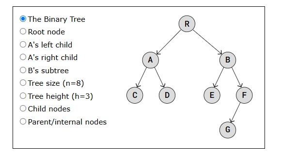
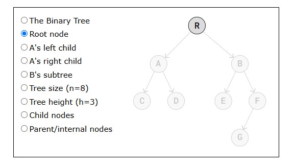
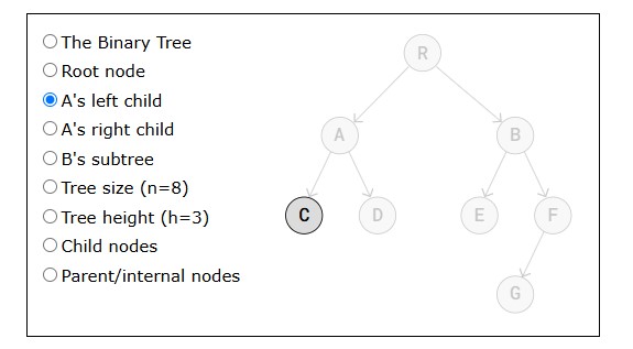
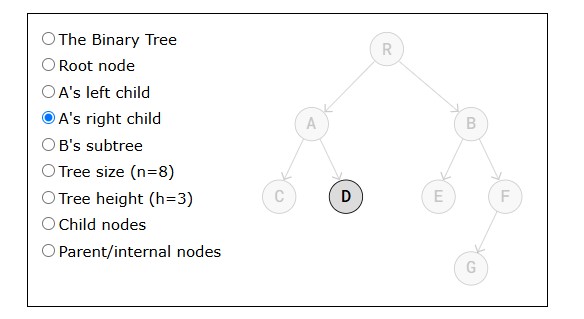
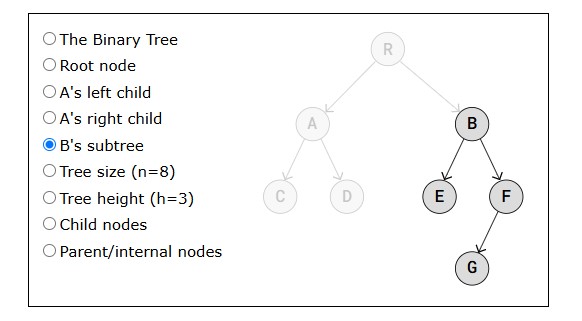
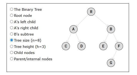
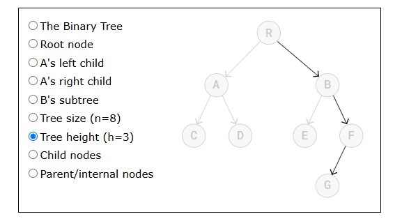
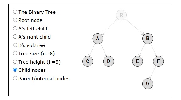
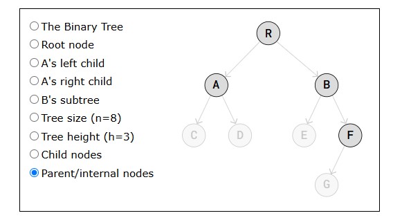
- A parent node, or internal node, in a Binary Tree is a node with one or two child nodes.
- The left child node is the child node to the left.
- The right child node is the child node to the right.
- The tree height is the maximum number of edges from the root node to a leaf node.
- Binary Trees vs. Arrays and Linked Lists
Benefits of Binary Trees over Arrays and Linked Lists:
- Arrays are fast when you want to access an element directly, like element number 700 in an array of 1000 elements for example. But inserting and deleting elements require other elements to shift in memory to make place for the new element, or to take the deleted elements place, and that is time consuming.
- Linked Lists are fast when inserting or deleting nodes, no memory shifting needed, but to access an element inside the list, the list must be traversed, and that takes time.
- Binary Trees, such as Binary Search Trees and AVL Trees, are great compared to Arrays and Linked Lists because they are BOTH fast at accessing a node, AND fast when it comes to deleting or inserting a node, with no shifts in memory needed.
- Types of Binary Trees
There are different variants, or types, of Binary Trees worth discussing to get a better understanding of how Binary Trees can be structured.
- A balanced Binary Tree has at most 1 in difference between its left and right subtree heights, for each node in the tree.
- A complete Binary Tree has all levels full of nodes, except the last level, which is can also be full, or filled from left to right. The properties of a complete Binary Tree means it is also balanced.
- A full Binary Tree is a kind of tree where each node has either 0 or 2 child nodes.
- A perfect Binary Tree has all leaf nodes on the same level, which means that all levels are full of nodes, and all internal nodes have two child nodes.The properties of a perfect Binary Tree means it is also full, balanced, and complete.
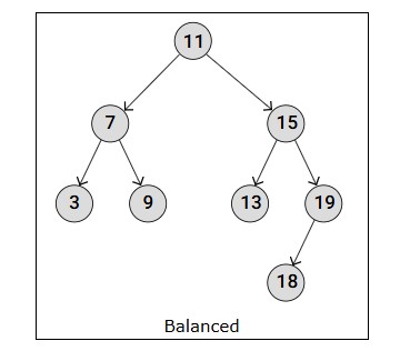
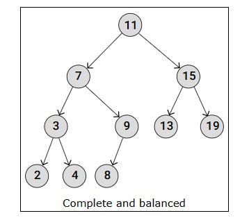
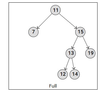
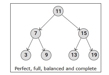
- Binary Tree Implementation
class TreeNode:
    def __init__(self, data):
        self.data = data
        self.left = None
        self.right = None

root = TreeNode('R')
nodeA = TreeNode('A')
nodeB = TreeNode('B')
nodeC = TreeNode('C')
nodeD = TreeNode('D')
nodeE = TreeNode('E')
nodeF = TreeNode('F')
nodeG = TreeNode('G')

root.left = nodeA
root.right = nodeB

nodeA.left = nodeC
nodeA.right = nodeD

nodeB.left = nodeE
nodeB.right = nodeF

nodeF.left = nodeG

# Test
print("root.right.left.data:", root.right.left.data)
- Binary Tree Traversal
Going through a Tree by visiting every node, one node at a time, is called traversal.
Since Arrays and Linked Lists are linear data structures, there is only one obvious way to traverse these: start at the first element, or node, and continue to visit the next until you have visited them all.
But since a Tree can branch out in different directions (non-linear), there are different ways of traversing Trees.
There are two main categories of Tree traversal methods:
Breadth First Search (BFS) is when the nodes on the same level are visited before going to the next level in the tree. This means that the tree is explored in a more sideways direction.
Depth First Search (DFS) is when the traversal moves down the tree all the way to the leaf nodes, exploring the tree branch by branch in a downwards direction.
There are three different types of DFS traversals:
- pre-order
- in-order
- post-order
Pre-order Traversal of Binary Trees
Pre-order Traversal is a type of Depth First Search, where each node is visited in a certain order.
Pre-order Traversal is done by visiting the root node first, then recursively do a pre-order traversal of the left subtree, followed by a recursive pre-order traversal of the right subtree. It's used for creating a copy of the tree, prefix notation of an expression tree, etc.
This traversal is "pre" order because the node is visited "before" the recursive pre-order traversal of the left and right subtrees.
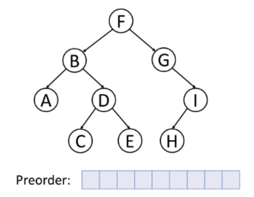
This is how the code for pre-order traversal looks like:
class TreeNode:
    def __init__(self, data):
        self.data = data
        self.left = None
        self.right = None

def preOrderTraversal(node):
    if node is None:
        return
    print(node.data, end=", ")
    preOrderTraversal(node.left)
    preOrderTraversal(node.right)

root = TreeNode('R')
nodeA = TreeNode('A')
nodeB = TreeNode('B')
nodeC = TreeNode('C')
nodeD = TreeNode('D')
nodeE = TreeNode('E')
nodeF = TreeNode('F')
nodeG = TreeNode('G')

root.left = nodeA
root.right = nodeB

nodeA.left = nodeC
nodeA.right = nodeD

nodeB.left = nodeE
nodeB.right = nodeF

nodeF.left = nodeG

# Traverse
preOrderTraversal(root)
In-order Traversal of Binary Trees
In-order Traversal is a type of Depth First Search, where each node is visited in a certain order.
In-order Traversal does a recursive In-order Traversal of the left subtree, visits the root node, and finally, does a recursive In-order Traversal of the right subtree. This traversal is mainly used for Binary Search Trees where it returns values in ascending order.
What makes this traversal "in" order, is that the node is visited in between the recursive function calls. The node is visited after the In-order Traversal of the left subtree, and before the In-order Traversal of the right subtree.
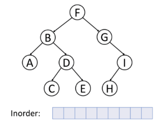
This is how the code for In-order Traversal looks like:
class TreeNode:
def __init__(self, data):
self.data = data
self.left = None
self.right = None
def inOrderTraversal(node):
if node is None:
return
inOrderTraversal(node.left)
print(node.data, end=", ")
inOrderTraversal(node.right)
root = TreeNode('R')
nodeA = TreeNode('A')
nodeB = TreeNode('B')
nodeC = TreeNode('C')
nodeD = TreeNode('D')
nodeE = TreeNode('E')
nodeF = TreeNode('F')
nodeG = TreeNode('G')
root.left = nodeA
root.right = nodeB
nodeA.left = nodeC
nodeA.right = nodeD
nodeB.left = nodeE
nodeB.right = nodeF
nodeF.left = nodeG
# Traverse
inOrderTraversal(root)
Post-order Traversal of Binary Trees
Post-order Traversal is a type of Depth First Search, where each node is visited in a certain order.
Post-order Traversal works by recursively doing a Post-order Traversal of the left subtree and the right subtree, followed by a visit to the root node. It is used for deleting a tree, post-fix notation of an expression tree, etc.
What makes this traversal "post" is that visiting a node is done "after" the left and right child nodes are called recursively.
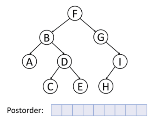
This is how the code for Post-order Traversal looks like:
class TreeNode:
    def __init__(self, data):
        self.data = data
        self.left = None
        self.right = None

def postOrderTraversal(node):
    if node is None:
        return
    postOrderTraversal(node.left)
    postOrderTraversal(node.right)
    print(node.data, end=", ")

root = TreeNode('R')
nodeA = TreeNode('A')
nodeB = TreeNode('B')
nodeC = TreeNode('C')
nodeD = TreeNode('D')
nodeE = TreeNode('E')
nodeF = TreeNode('F')
nodeG = TreeNode('G')

root.left = nodeA
root.right = nodeB

nodeA.left = nodeC
nodeA.right = nodeD

nodeB.left = nodeE
nodeB.right = nodeF

nodeF.left = nodeG

# Traverse
postOrderTraversal(root)
Graphs
A Graph is a non-linear data structure that consists of vertices (nodes) and edges.
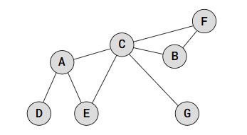
A vertex, also called a node, is a point or an object in the Graph, and an edge is used to connect two vertices with each other.
Graphs are non-linear because the data structure allows us to have different paths to get from one vertex to another, unlike with linear data structures like Arrays or Linked Lists.
Graphs are used to represent and solve problems where the data consists of objects and relationships between them, such as:
- Social Networks: Each person is a vertex, and relationships (like friendships) are the edges. Algorithms can suggest potential friends.
- Maps and Navigation: Locations, like a town or bus stops, are stored as vertices, and roads are stored as edges. Algorithms can find the shortest route between two locations when stored as a Graph.
- Internet: Can be represented as a Graph, with web pages as vertices and hyperlinks as edges.
- Biology: Graphs can model systems like neural networks or the spread of diseases.
- Graph Properties
A weighted Graph is a Graph where the edges have values. The weight value of an edge can represent things like distance, capacity, time, or probability.
A connected Graph is when all the vertices are connected through edges somehow. A Graph that is not connected, is a Graph with isolated (disjoint) subgraphs, or single isolated vertices.
A directed Graph, also known as a digraph, is when the edges between the vertex pairs have a direction. The direction of an edge can represent things like hierarchy or flow.
A cyclic Graph is defined differently depending on whether it is directed or not:
- A directed cyclic Graph is when you can follow a path along the directed edges that goes in circles.
- An undirected cyclic Graph is when you can come back to the same vertex you started at without using the same edge more than once.
A loop, also called a self-loop, is an edge that begins and ends on the same vertex. A loop is a cycle that only consists of one edge.
- Graph Representations
A Graph representation tells us how a Graph is stored in memory.
Different Graph representations can:
- take up more or less space.
- be faster or slower to search or manipulate.
- be better suited depending on what type of Graph we have (weighted, directed, etc.), and what we want to do with the Graph.
- be easier to understand and implement than others.
Graph representations store information about which vertices are adjacent, and how the edges between the vertices are. Graph representations are slightly different if the edges are directed or weighted.
Two vertices are adjacent, or neighbors, if there is an edge between them.
- Adjacency Matrix Graph Representation
The Adjacency Matrix is a 2D array (matrix) where each cell on index (i, j) stores information about the edge from vertex i to vertex j.
Below is a Graph with the Adjacency Matrix representation next to it.
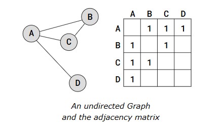
The adjacency matrix above represents an undirected Graph, so the values '1' only tells us where the edges are. Also, the values in the adjacency matrix is symmetrical because the edges go both ways (undirected Graph).
To create a directed Graph with an adjacency matrix, we must decide which vertices the edges go from and to, by inserting the value at the correct indexes (i, j). To represent a weighted Graph we can put other values than '1' inside the adjacency matrix.
Below is a directed and weighted Graph with the Adjacency Matrix representation next to it.
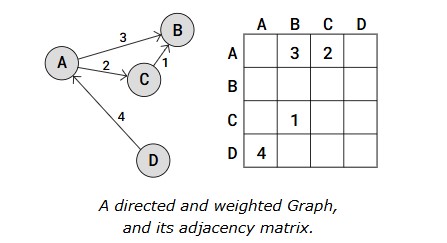
In the adjacency matrix above, the value 3 on index (0, 1) tells us there is an edge from vertex A to vertex B, and the weight for that edge is 3.
As you can see, the weights are placed directly into the adjacency matrix for the correct edge, and for a directed Graph, the adjacency matrix does not have to be symmetric.
- Adjacency List Graph Representation
In case we have a 'sparse' Graph with many vertices, we can save space by using an Adjacency List compared to using an Adjacency Matrix, because an Adjacency Matrix would reserve a lot of memory on empty Array elements for edges that don't exist.
A 'sparse' Graph is a Graph where each vertex only has edges to a small portion of the other vertices in the Graph.
An Adjacency List has an array that contains all the vertices in the Graph, and each vertex has a Linked List (or Array) with the vertex's edges.
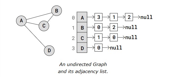
In the adjacency list above, the vertices A to D are placed in an Array, and each vertex in the array has its index written right next to it.
Each vertex in the Array has a pointer to a Linked List that represents that vertex's edges. More specifically, the Linked List contains the indexes to the adjacent (neighbor) vertices.
So for example, vertex A has a link to a Linked List with values 3, 1, and 2. These values are the indexes to A's adjacent vertices D, B, and C.
An Adjacency List can also represent a directed and weighted Graph, like this:
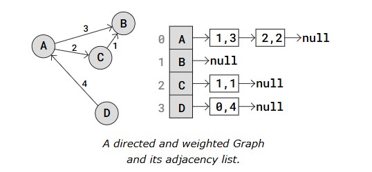
In the Adjacency List above, vertices are stored in an Array. Each vertex has a pointer to a Linked List with edges stored as i,w, where i is the index of the vertex the edge goes to, and w is the weight of that edge.
Node D for example, has a pointer to a Linked List with an edge to vertex A. The values 0,4 means that vertex D has an edge to vertex on index 0 (vertex A), and the weight of that edge is 4.
Shortest Path
- The Shortest Path Problem
The shortest path problem is famous in the field of computer science.
To solve the shortest path problem means to find the shortest possible route or path between two vertices (or nodes) in a Graph.
In the shortest path problem, a Graph can represent anything from a road network to a communication network, where the vertices can be intersections, cities, or routers, and the edges can be roads, flight paths, or data links.
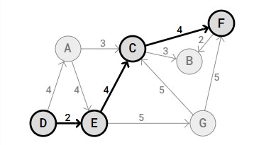
The shortest path from vertex D to vertex F in the Graph above is D->E->C->F, with a total path weight of 2+4+4=10. Other paths from D to F are also possible, but they have a higher total weight, so they can not be considered to be the shortest path.
- Solutions to The Shortest Path Problem
Dijkstra's algorithm and the Bellman-Ford algorithm find the shortest path from one start vertex, to all other vertices.
To solve the shortest path problem means to check the edges inside the Graph until we find a path where we can move from one vertex to another using the lowest possible combined weight along the edges.
This sum of weights along the edges that make up a path is called a path cost or a path weight.
Algorithms that find the shortest paths, like Dijkstra's algorithm or the Bellman-Ford algorithm, find the shortest paths from one start vertex to all other vertices.
To begin with, the algorithms set the distance from the start vertex to all vertices to be infinitely long. And as the algorithms run, edges between the vertices are checked over and over, and shorter paths might be found many times until the shortest paths are found at the end.
Every time an edge is checked and it leads to a shorter distance to a vertex being found and updated, it is called a relaxation, or relaxing an edge.
- Positive and Negative Edge Weights
Some algorithms that find the shortest paths, like Dijkstra's algorithm, can only find the shortest paths in graphs where all the edges are positive. Such graphs with positive distances are also the easiest to understand because we can think of the edges between vertices as distances between locations.
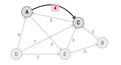
If we interpret the edge weights as money lost by going from one vertex to another, a positive edge weight of 4 from vertex A to C in the graph above means that we must spend $4 to go from A to C.
But graphs can also have negative edges, and for such graphs the Bellman-Ford algorithm can be used to find the shortest paths.
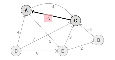
And similarly, if the edge weights represent money lost, the negative edge weight -3 from vertex C to A in the graph above can be understood as an edge where there is more money to be made than money lost by going from C to A. So if for example the cost of fuel is $5 going from C to A, and we get paid $8 for picking up packages in C and delivering them in A, money lost is -3, meaning we are actually earning $3 in total.
- Negative Cycles in Shortest Path Problems
Finding the shortest paths becomes impossible if a graph has negative cycles.
Having a negative cycle means that there is a path where you can go in circles, and the edges that make up this circle have a total path weight that is negative.
In the graph below, the path A->E->B->C->A is a negative cycle because the total path weight is 5+2-4-4=-1.
The reason why it is impossible to find the shortest paths in a graph with negative cycles is that it will always be possible to continue running an algorithm to find even shorter paths.
Let's say for example that we are looking for the shortest distance from vertex D in graph above, to all other vertices. At first we find the distance from D to E to be 3, by just walking the edge D->E. But after this, if we walk one round in the negative cycle E->B->C->A->E, then the distance to E becomes 2. After walking one more round the distance becomes 1, which is even shorter, and so on. We can always walk one more round in the negative cycle to find a shorter distance to E, which means the shortest distance can never be found.
Luckily, the the Bellman-Ford algorithm, that runs on graphs with negative edges, can be implemented with detection for negative cycles.
Minimum Spanning Tree
The Minimum Spanning Tree (MST) is the collection of edges required to connect all vertices in an undirected graph, with the minimum total edge weight.
It is called a Minimum Spanning Tree, because it is a connected, acyclic, undirected graph, which is the definition of a tree data structure.
In the real world, finding the Minimum Spanning Tree can help us find the most effective way to connect houses to the internet or to the electrical grid, or it can help us finding the fastest route to deliver packages.
- MST Algorithms
Algorithms that finds the Minimum Spanning Tree in a graph: Prim's algorithm, and Kruskal's algorithm.
Source: W3